Stacking With Workflow Sets

The stacks package provides a shorthand interface for supplying multiple sets of candidate members in one call to add_candidates() via the workflowsets package. Instead of iteratively calling add_candidates() for each tuning result:

stacks() %>%
  add_candidates(tuning_result_1) %>%
  add_candidates(tuning_result_2) %>%
  add_candidates(tuning_result_3) %>%
  add_candidates(tuning_result_4) %>%
  blend_predictions() %>%
  fit_members()

…we can add candidate members “in batch:”

stacks() %>%
  add_candidates(wf_set) %>%
  blend_predictions() %>%
  fit_members()

This interface is especially helpful with a large number of candidate members, which is exactly the setting that model stacking excels in.

Setup

This example will parallel the “Getting Started” vignette, except that we will use workflowsets to bundle the model workflows that define the candidate members into one workflow set. We will then train each of them using workflowsets::workflow_map() and add the results to a model stack using add_candidates(). If you’re not familiar with the stacks package, refer to that vignette for the big picture!

First, loading needed packages:

library(tidymodels)
library(stacks)

In this example, we’ll again make use of the tree_frogs data exported with stacks, giving experimental results on hatching behavior of red-eyed tree frog embryos!

Red-eyed tree frog (RETF) embryos can hatch earlier than their normal 7ish days if they detect potential predator threat. Researchers wanted to determine how, and when, these tree frog embryos were able to detect stimulus from their environment. To do so, they subjected the embryos at varying developmental stages to “predator stimulus” by jiggling the embryos with a blunt probe. Beforehand, though some of the embryos were treated with gentamicin, a compound that knocks out their lateral line (a sensory organ.) Researcher Julie Jung and her crew found that these factors inform whether an embryo hatches prematurely or not!

We’ll start out with predicting latency (i.e. time to hatch) based on other attributes. We’ll need to filter out NAs (i.e. cases where the embryo did not hatch) first.

data("tree_frogs")

# subset the data
tree_frogs <- tree_frogs %>%
  filter(!is.na(latency)) %>%
  select(-c(clutch, hatched))

Taking a quick look at the data, it seems like the hatch time is pretty closely related to some of our predictors!

theme_set(theme_bw())

ggplot(tree_frogs) +
  aes(x = age, y = latency, color = treatment) +
  geom_point() +
  labs(x = "Embryo Age (s)", y = "Time to Hatch (s)", col = "Treatment")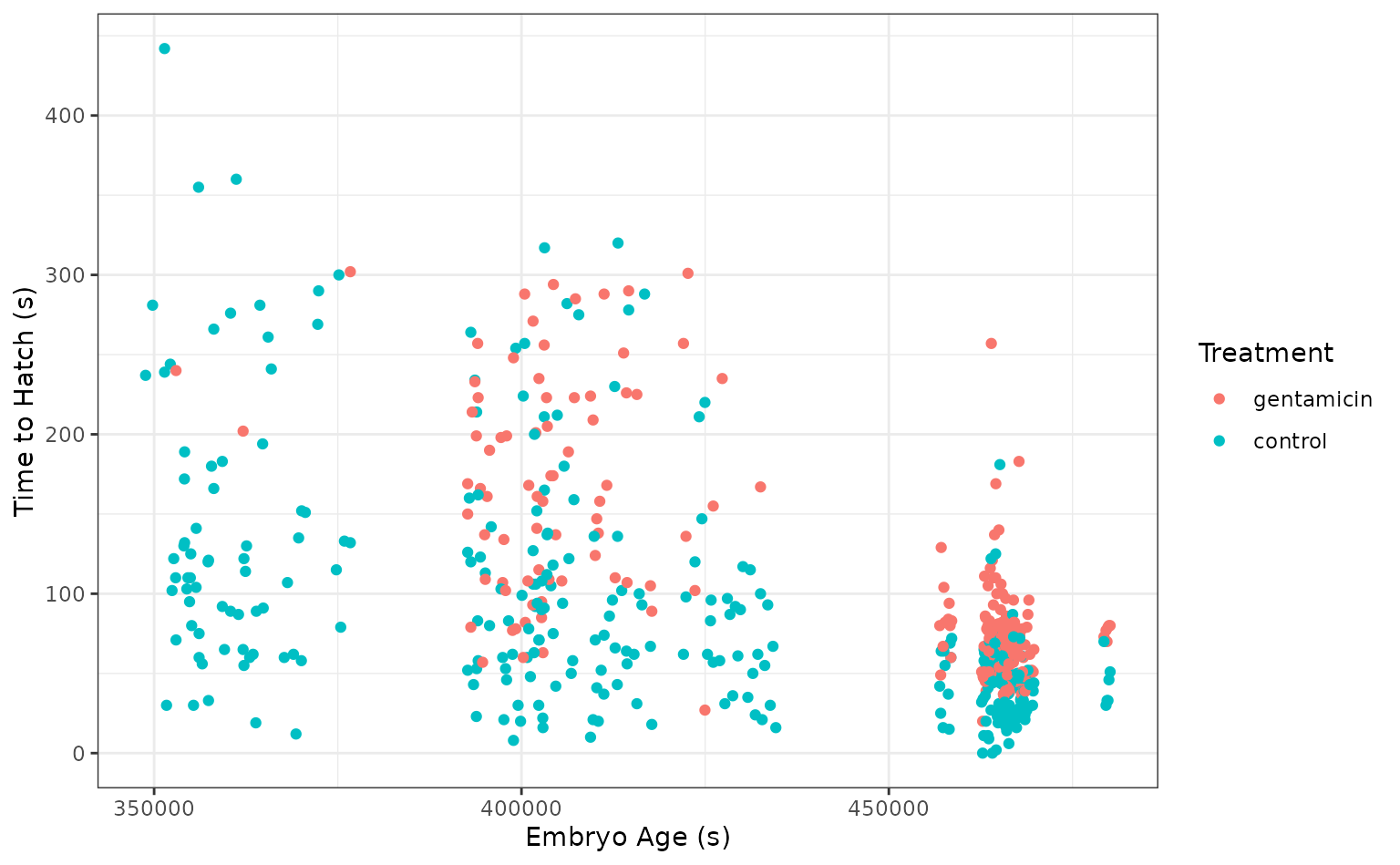

Let’s give this a go!

Defining candidate ensemble members

As in the workflow-based setting, defining the candidate ensemble members is undoubtedly the longest part of the ensembling process with stacks. Instead of evaluating our model specifications via resampling for each workflow, though, we combine each of the model specifications with workflow_set(), and then evaluate them in batch with the workflow_map() function.

First, splitting up the training data, generating resamples, and setting some options that will be used by each model definition:

# some setup: resampling and a basic recipe
set.seed(1)
tree_frogs_split <- initial_split(tree_frogs)
tree_frogs_train <- training(tree_frogs_split)
tree_frogs_test  <- testing(tree_frogs_split)

set.seed(1)
folds <- rsample::vfold_cv(tree_frogs_train, v = 5)

tree_frogs_rec <- 
  recipe(latency ~ ., data = tree_frogs_train)

metric <- metric_set(rmse)

We also need to use the same control settings as in the workflow-based setting:

ctrl_grid <- control_stack_grid()

We’ll define three different model definitions to try to predict time to hatch—a K-nearest neighbors model (with hyperparameters to tune), a linear model, and a support vector machine model (again, with hyperparameters to tune).

Starting out with K-nearest neighbors, we begin by creating a parsnip model specification:

# create a model specification
knn_spec <-
  nearest_neighbor(
    mode = "regression", 
    neighbors = tune("k")
  ) %>%
  set_engine("kknn")

knn_spec
#> K-Nearest Neighbor Model Specification (regression)
#> 
#> Main Arguments:
#>   neighbors = tune("k")
#> 
#> Computational engine: kknn

Note that, since we are tuning over several possible numbers of neighbors, this model specification defines multiple model configurations. The specific form of those configurations will be determined when specifying the grid search.

From here, we extend the basic recipe defined earlier to fully specify the form of the design matrix for use in a K-nearest neighbors model:

# extend the recipe
knn_rec <-
  tree_frogs_rec %>%
  step_dummy(all_nominal_predictors()) %>%
  step_zv(all_predictors()) %>%
  step_impute_mean(all_numeric_predictors()) %>%
  step_normalize(all_numeric_predictors())

knn_rec
#> 
#> ── Recipe ────────────────────────────────────────────────────────────────
#> 
#> ── Inputs
#> Number of variables by role
#> outcome:   1
#> predictor: 4
#> 
#> ── Operations
#> • Dummy variables from: all_nominal_predictors()
#> • Zero variance filter on: all_predictors()
#> • Mean imputation for: all_numeric_predictors()
#> • Centering and scaling for: all_numeric_predictors()

Starting with the basic recipe, we convert categorical predictors to dummy variables, remove predictors with only one observation, impute missing values in numeric predictors using the mean, and normalize numeric predictors. Pre-processing instructions for the remaining models are defined similarly.

Now, specifying the linear model, note that we are not optimizing over any hyperparameters.

# create a model specification
lin_reg_spec <-
  linear_reg() %>%
  set_engine("lm")

# extend the recipe
lin_reg_rec <-
  tree_frogs_rec %>%
  step_dummy(all_nominal_predictors()) %>%
  step_zv(all_predictors())

Finally, putting together the model specification and recipe for the support vector machine:

# create a model specification
svm_spec <- 
  svm_rbf(
    cost = tune("cost"), 
    rbf_sigma = tune("sigma")
  ) %>%
  set_engine("kernlab") %>%
  set_mode("regression")

# extend the recipe
svm_rec <-
  tree_frogs_rec %>%
  step_dummy(all_nominal_predictors()) %>%
  step_zv(all_predictors()) %>%
  step_impute_mean(all_numeric_predictors()) %>%
  step_corr(all_predictors()) %>%
  step_normalize(all_numeric_predictors())

With each model specification and accompanying recipe now defined, we can combine them via workflow_set:

wf_set <- 
  workflow_set(
    preproc = list(rec1 = knn_rec, rec2 = lin_reg_rec,     rec3 = svm_rec),
    models =  list(knn = knn_spec, lin_reg = lin_reg_spec, svm = svm_spec),
    cross = FALSE
  )

wf_set
#> # A workflow set/tibble: 3 × 4
#>   wflow_id     info             option    result    
#>   <chr>        <list>           <list>    <list>    
#> 1 rec1_knn     <tibble [1 × 4]> <opts[0]> <list [0]>
#> 2 rec2_lin_reg <tibble [1 × 4]> <opts[0]> <list [0]>
#> 3 rec3_svm     <tibble [1 × 4]> <opts[0]> <list [0]>

Note that each combination of preprocessor and model specification is assigned a wflow_id that we can use to interface with individual model definitions:

wf_set %>%
  extract_workflow("rec3_svm")
#> ══ Workflow ══════════════════════════════════════════════════════════════
#> Preprocessor: Recipe
#> Model: svm_rbf()
#> 
#> ── Preprocessor ──────────────────────────────────────────────────────────
#> 5 Recipe Steps
#> 
#> • step_dummy()
#> • step_zv()
#> • step_impute_mean()
#> • step_corr()
#> • step_normalize()
#> 
#> ── Model ─────────────────────────────────────────────────────────────────
#> Radial Basis Function Support Vector Machine Model Specification (regression)
#> 
#> Main Arguments:
#>   cost = tune("cost")
#>   rbf_sigma = tune("sigma")
#> 
#> Computational engine: kernlab

The elements in this workflow set are nearly ready to be evaluated with tune_grid(). Before we do so, though, we need to ensure that we fit each with the appropriate control options, just as we do when evaluating individual workflows on resamples before passing them to stacks.

We can iteratively add the appropriate control settings with the control_stack_grid() shorthand using the option_add() function:

wf_set <-
  wf_set %>%
  option_add(
    control = control_stack_grid(),
    metrics = metric
  )

We can now use the workflow_map() function to map over each model definition, evaluating hyperparameters on the supplied resamples.

wf_set_trained <-
  workflow_map(
    wf_set,
    fn = "tune_grid",
    resamples = folds
  )

wf_set_trained
#> # A workflow set/tibble: 3 × 4
#>   wflow_id     info             option    result   
#>   <chr>        <list>           <list>    <list>   
#> 1 rec1_knn     <tibble [1 × 4]> <opts[3]> <tune[+]>
#> 2 rec2_lin_reg <tibble [1 × 4]> <opts[3]> <rsmp[+]>
#> 3 rec3_svm     <tibble [1 × 4]> <opts[3]> <tune[+]>

The results section now contains three sets of tuning results. Note that the results corresponding to the linear regression have the subclass resample_results rather than tune_results—this is expected, as there were no hyperparameters to tune for that model specification. workflow_map() knows to fall back to fit_resamples() rather than tune_grid(), in this case!

We can extract tuning results with the extract_workflow_set_result() helper to explore our tuning results:

extract_workflow_set_result(wf_set_trained, id = "rec1_knn") %>%
  collect_metrics(summarize = TRUE)
#> # A tibble: 10 × 7
#>        k .metric .estimator  mean     n std_err .config              
#>    <int> <chr>   <chr>      <dbl> <int>   <dbl> <chr>                
#>  1     1 rmse    standard    81.3     5    4.37 Preprocessor1_Model01
#>  2     3 rmse    standard    69.6     5    3.57 Preprocessor1_Model02
#>  3     5 rmse    standard    63.7     5    3.30 Preprocessor1_Model03
#>  4     6 rmse    standard    62.3     5    3.12 Preprocessor1_Model04
#>  5     7 rmse    standard    61.2     5    2.95 Preprocessor1_Model05
#>  6     9 rmse    standard    59.8     5    2.82 Preprocessor1_Model06
#>  7    10 rmse    standard    59.3     5    2.83 Preprocessor1_Model07
#>  8    11 rmse    standard    59.0     5    2.82 Preprocessor1_Model08
#>  9    13 rmse    standard    58.5     5    2.84 Preprocessor1_Model09
#> 10    15 rmse    standard    58.2     5    2.88 Preprocessor1_Model10

With these three model definitions fully specified and tuned in a workflow set, we are ready to begin stacking these model configurations. (Note that, in most applied settings, one would likely specify many more than a handful candidate members from three model definitions.)

Putting together a stack

Building the stacked ensemble, now, takes even fewer lines than it did with individual workflows:

tree_frogs_model_st <- 
  # initialize the stack
  stacks() %>%
  # add candidate members
  add_candidates(wf_set_trained) %>%
  # determine how to combine their predictions
  blend_predictions() %>%
  # fit the candidates with nonzero stacking coefficients
  fit_members()

tree_frogs_model_st
#> # A tibble: 4 × 3
#>   member           type             weight
#>   <chr>            <chr>             <dbl>
#> 1 rec3_svm_1_06    svm_rbf          0.779 
#> 2 rec2_lin_reg_1_1 linear_reg       0.275 
#> 3 rec1_knn_1_08    nearest_neighbor 0.190 
#> 4 rec1_knn_1_07    nearest_neighbor 0.0205

The results obtained from building a model stack with workflow sets are identical to those that would result from building a model stack with individual workflows.

To make sure that we have the right trade-off between minimizing the number of members and optimizing performance, we can use:

autoplot(tree_frogs_model_st)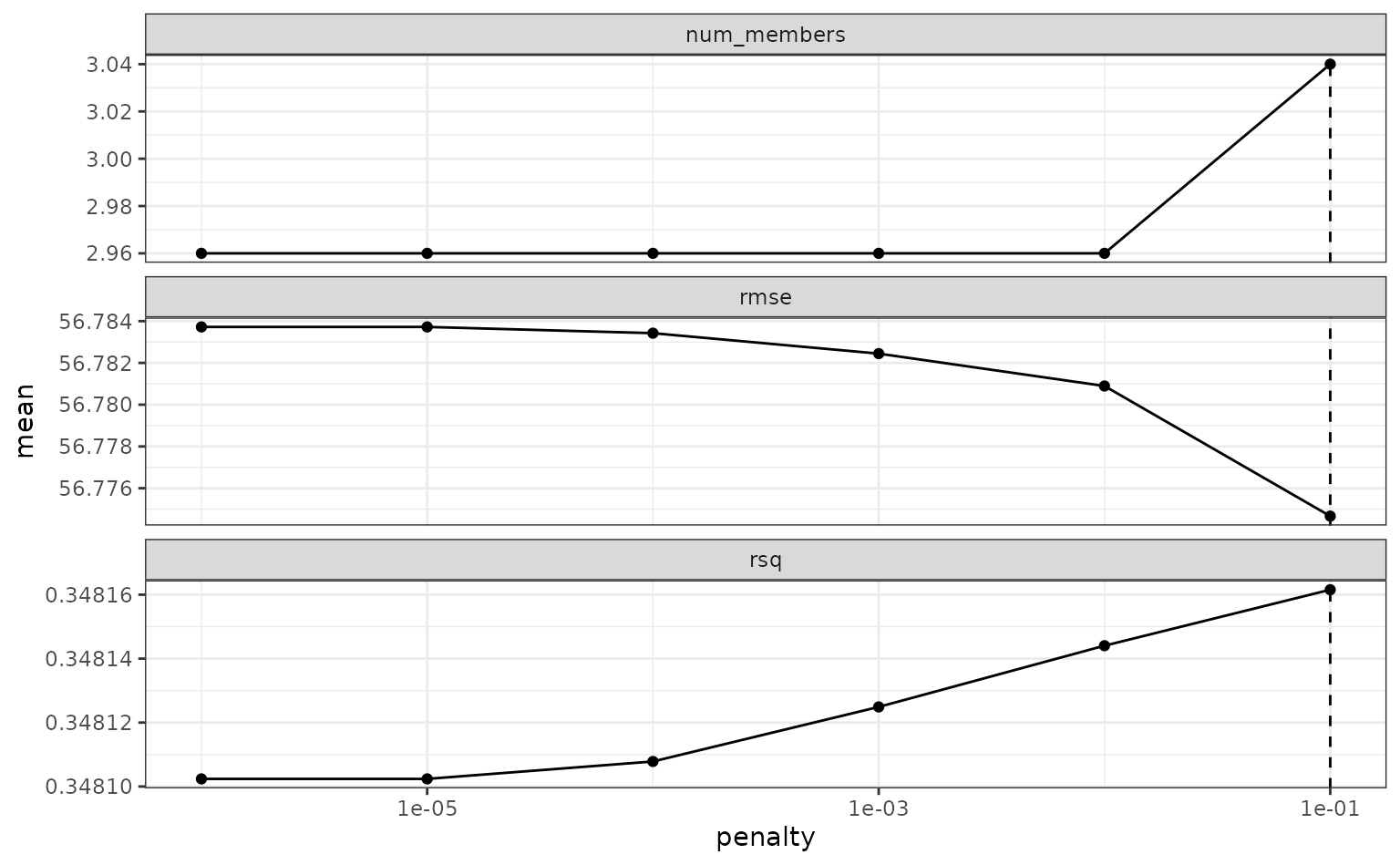

If these results were not good enough, blend_predictions() could be called again with different values of penalty. As it is, blend_predictions() picks the penalty parameter with the numerically optimal results. To see the top results:

autoplot(tree_frogs_model_st, type = "weights")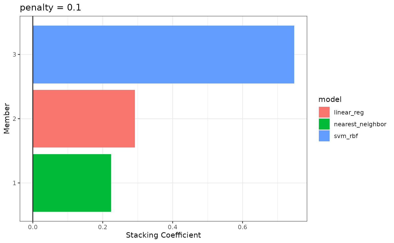

To identify which model configurations were assigned what stacking coefficients, we can make use of the collect_parameters() function:

collect_parameters(tree_frogs_model_st, "rec3_svm")
#> # A tibble: 10 × 4
#>    member            cost    sigma  coef
#>    <chr>            <dbl>    <dbl> <dbl>
#>  1 rec3_svm_1_01  0.185   1.17e- 4 0    
#>  2 rec3_svm_1_02  1.23    2.39e- 7 0    
#>  3 rec3_svm_1_03  0.0195  3.37e- 5 0    
#>  4 rec3_svm_1_04 15.2     4.78e- 8 0    
#>  5 rec3_svm_1_05  2.97    1.30e- 6 0    
#>  6 rec3_svm_1_06  0.134   5.62e- 2 0.779
#>  7 rec3_svm_1_07  0.00163 3.01e- 3 0    
#>  8 rec3_svm_1_08  4.08    2.98e- 1 0    
#>  9 rec3_svm_1_09  0.00429 3.45e-10 0    
#> 10 rec3_svm_1_10  0.0280  1.54e- 9 0

This object is now ready to predict with new data!

tree_frogs_test <- 
  tree_frogs_test %>%
  bind_cols(predict(tree_frogs_model_st, .))

Juxtaposing the predictions with the true data:

ggplot(tree_frogs_test) +
  aes(x = latency, 
      y = .pred) +
  geom_point() + 
  coord_obs_pred()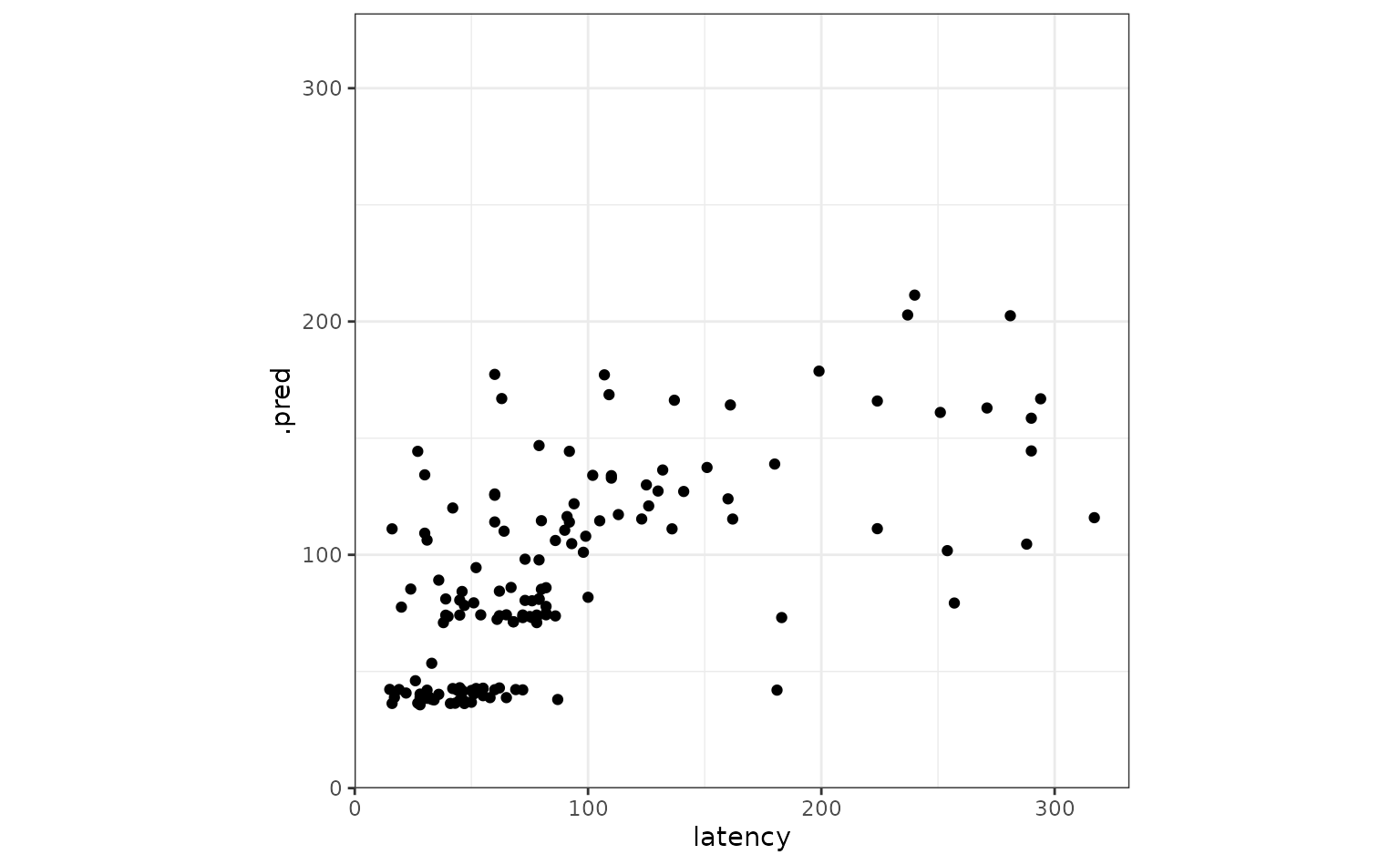

Looks like our predictions were decent! How do the stacks predictions perform, though, as compared to the members’ predictions? We can use the type = "members" argument to generate predictions from each of the ensemble members.

member_preds <- 
  tree_frogs_test %>%
  select(latency) %>%
  bind_cols(predict(tree_frogs_model_st, tree_frogs_test, members = TRUE))

Now, evaluating the root mean squared error from each model:

map(member_preds, rmse_vec, truth = member_preds$latency) %>%
  as_tibble()
#> # A tibble: 1 × 6
#>   latency .pred rec1_knn_1_07 rec1_knn_1_08 rec2_lin_reg_1_1 rec3_svm_1_06
#>     <dbl> <dbl>         <dbl>         <dbl>            <dbl>         <dbl>
#> 1       0  53.9          56.2          56.2             55.5          57.3

As we can see, the stacked ensemble outperforms each of the member models, though is closely followed by one of its members.

Voila! You’ve now made use of the stacks and workflowsets packages to predict red-eyed tree frog embryo hatching using a stacked ensemble!